DataFrame and Simple Linear Regression
In the previous post I mentioned using Iceberg successfully. The code I was pushing is SLRCalculator, a simple linear regression calculator, written to take Oleksandr Zaytsev's DataFrame library for a spin, by way of porting Jason Brownlee's excellent simple linear regression in Python to Pharo.
Firstly, install DataFrame. This also pulls in Roassal.
Metacello new
  baseline: 'DataFrame';
  repository: 'github://PolyMathOrg/DataFrame';
  load.
SLRCalculator implements mean, variance, covariance, coefficients etc, and also incorporates the Swedish automobile insurance dataset used by Jason in his Python example.
SLRCalculator class>>loadSwedishAutoInsuranceData
  "Source: https://www.math.muni.cz/~kolacek/docs/frvs/M7222/data/AutoInsurSweden.txt"
  | df |

  df := DataFrame fromRows: #(
            ( 108 392.5 )
            ( 19 46.2 )
            ( 13 15.7 )
            "more lines" ).
  df columnNames: #(X Y).
  ^ df
The computation for covariance also uses DataFrame.
covariance: dataFrame
  | xvalues yvalues xmean ymean covar |

  xvalues := dataFrame columnAt: 1.
  yvalues := dataFrame columnAt: 2.
  xmean := self mean: xvalues.
  ymean := self mean: yvalues.
  covar := 0.
  1 to: xvalues size do: [ :idx |
    covar := covar + (((xvalues at: idx) - xmean) * ((yvalues at: idx) - ymean)) ].
  ^ covar
Let's see how to use SLRCalculator to perform linear regression, with graphing using Roassal. First declare the variables and instantiate some objects:
| allData splitArray trainingData testData s coeff g dsa dlr legend |

s := SLRCalculator new.

allData := SLRCalculator loadSwedishAutoInsuranceData.
Next, split the data set into training and test subsets. Splitting without shuffling means to always take the first 60% of the data for training.
splitArray := s extractForTesting: allData by: 60 percent shuffled: false.
trainingData := splitArray at: 1.
testData := splitArray at: 2.
coeff := s coefficients: trainingData.
Set up for graphing. Load `allData' as points.
g := RTGrapher new.

allData do: [ :row |
  dsa := RTData new.
  dsa dotShape color: Color blue.
  dsa points: { (row at: 1) @ (row at: 2) }.
  dsa x: #x.
  dsa y: #y.
  g add: dsa ].
Create the points to plot the linear regression of the full data set, using the coefficients computed from the training subset.
dlr := RTData new.
dlr noDot.
dlr connectColor: Color red.
dlr points: (allData column: #X).
" y = b0 + (b1 * x) "
dlr x: #yourself.
dlr y: [ :v | (coeff at: 1) + (v * (coeff at: 2)) ].
g add: dlr.
Make the plot look nice.
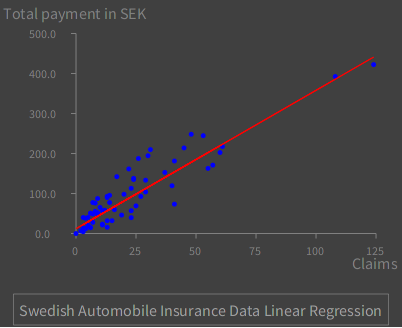
g axisX noDecimal; title: 'Claims'.
g axisY title: 'Total payment in SEK'.
g shouldUseNiceLabels: true.
g build.

legend := RTLegendBuilder new.
legend view: g view.
legend addText: 'Swedish Automobile Insurance Data Linear Regression'.
legend build.

g view
Putting the code altogether:
| allData splitArray trainingData testData s coeff g dsa dlr legend |

s := SLRCalculator new.

allData := SLRCalculator loadSwedishAutoInsuranceData.
splitArray := s extractForTesting: allData by: 60 percent shuffled: false.
trainingData := splitArray at: 1.
testData := splitArray at: 2.
coeff := s coefficients: trainingData.

g := RTGrapher new.

allData do: [ :row |
  dsa := RTData new.
  dsa dotShape color: Color blue.
  dsa points: { (row at: 1) @ (row at: 2) }.
  dsa x: #x.
  dsa y: #y.
  g add: dsa ].

dlr := RTData new.
dlr noDot.
dlr connectColor: Color red.
dlr points: (allData column: #X).
" y = b0 + (b1 * x) "
dlr x: #yourself.
dlr y: [ :v | (coeff at: 1) + (v * (coeff at: 2)) ].
g add: dlr.

g axisX noDecimal; title: 'Claims'.
g axisY title: 'Total payment in SEK'.
g shouldUseNiceLabels: true.
g build.

legend := RTLegendBuilder new.
legend view: g view.
legend addText: 'Swedish Automobile Insurance Data Linear Regression'.
legend build.

g view
Copy/paste the code into a playground, press shift-ctrl-g...